Mastering Contour Plots & 3D Visualizations in Python and MATLAB for Q1 Journals
A practical walkthrough for PhD scholars and engineering authors.

Reviewers look at your figures before they read your text. A clean contour plot or a well-built 3D surface can make a result obvious in seconds. A cluttered one can make a good result look doubtful. Good figures follow one simple rule: every element should help the reader read a value, not decorate the page. Fig. 1 shows the same data twice, with the default look on the left and a publication-ready version on the right.
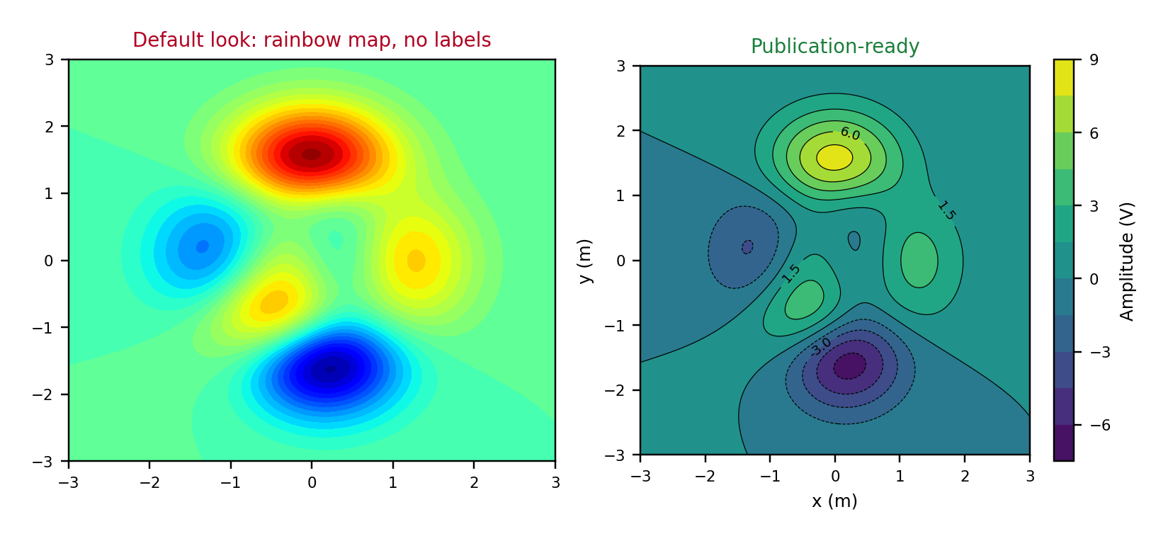
Fig. 1. The same data: default rainbow plot versus a publication-ready contour plot.
This guide covers the full routine in Python (Matplotlib and NumPy) and MATLAB: choosing the plot type, preparing data, building readable contours, picking color maps, making clean 3D surfaces, and exporting for top-quartile (Q1) journals. Every Python snippet below was run to produce the figures you see.
Step 1: Choose the Right Plot Type
Start with the question the figure answers. A reader who needs to read values wants contours. A reader who needs the overall shape may be happy with a surface.
| Plot | Best for | Watch out for |
|---|---|---|
| Contour lines | Reading levels and comparing curves | Too many levels, unlabeled lines |
| Filled contour | Magnitude and shape together | Misleading color maps |
| Heat map | Raw gridded data, no smoothing | Blocky cells on coarse grids |
| 3D surface | Peaks, valleys, saddles | Hidden regions, hard to read values |
| 3D scatter or path | Trajectories and point clouds | Depth ambiguity |
A safe rule: if a 2D plot tells the same story, use the 2D plot. Use 3D when the third dimension adds understanding, and pair it with a contour projection or a 2D slice so readers can still read values (Fig. 2).
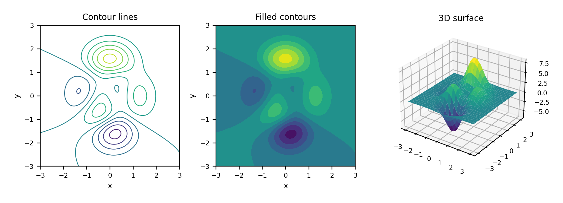
Fig. 2. One function shown as contour lines, filled contours, and a 3D surface.
Step 2: Prepare Your Data
- Build a regular grid with meshgrid and keep units consistent throughout.
- For scattered measurements, interpolate onto a grid and state the method in the paper.
- Choose grid density from the data's real resolution. Over-smoothing can invent features that are not there.
- Keep the original points visible as markers when you can (Fig. 6).
Step 3: Build a Contour Plot That Reads Well
- Use about 10 to 15 evenly spaced levels. More lines add noise, not information.
- Combine filled contours with thin black lines, and label only some of the lines.
- Add a colorbar with a label and units, and label both axes with units.
- Use equal aspect ratio when x and y share the same unit.
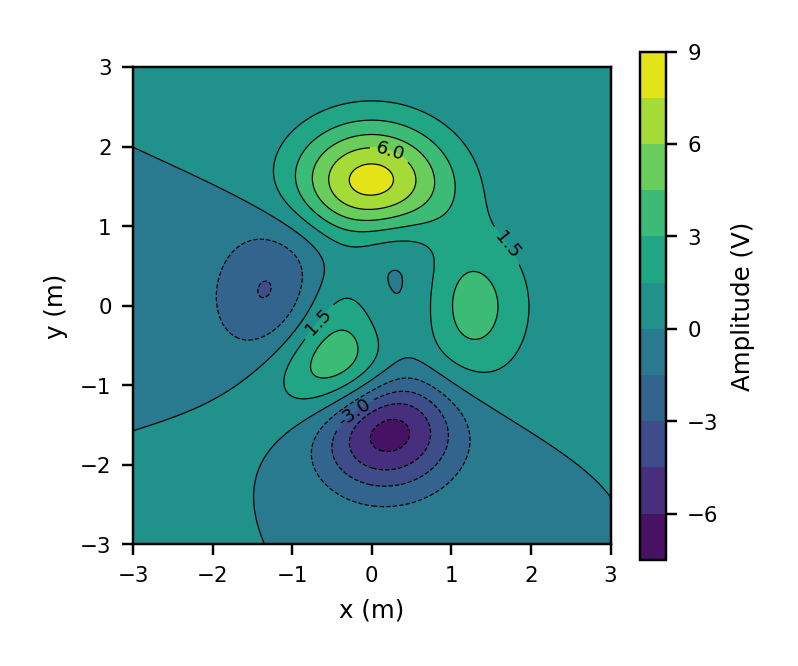
Fig. 3. Output of the Python code above at single-column width (3.5 in).
Step 4: Choose Color Maps Carefully
Color is where most figures go wrong. Rainbow maps such as jet create false boundaries, hide real detail, and turn into misleading bands in grayscale. Use perceptually uniform maps: viridis or cividis in Python, parula in MATLAB. The cividis map was designed with color vision deficiency in mind. Use diverging maps only for signed data, and center them at zero. Avoid red-green pairs, and run a grayscale test before submitting (Fig. 4).
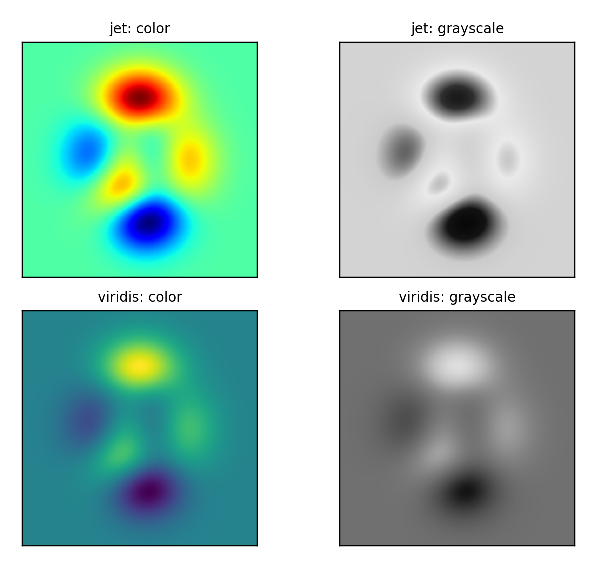
Fig. 4. Grayscale test: jet loses its order, while viridis keeps a smooth light-to-dark ramp.
Step 5: Make Clean 3D Surfaces
- Pick a viewing angle that hides nothing. An elevation of 25 to 35 degrees and an azimuth near -55 works for many peaks.
- Label all three axes with units, and lighten the grid and panes.
- Use smooth shading and no heavy black mesh. Check the surface from two angles before you commit.
- Keep the same view angle across panels that readers compare.
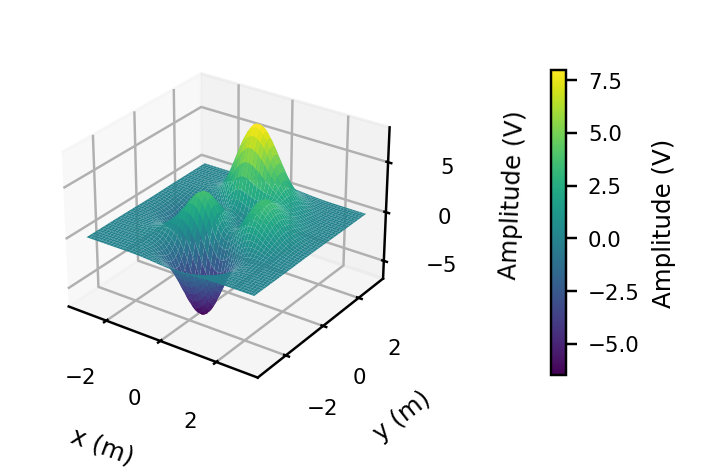
Fig. 5. A clean 3D surface: clear angle, labeled axes, smooth shading, and a colorbar.
Step 6: Overlay Data, Paths, and Optima
Overlays turn a plot into evidence. Add measurements as markers, optimization paths as lines, and the optimum as a distinct symbol with a legend entry (Fig. 6). Use black or white overlays with an outline so they stay visible on any color. For functions that span several orders of magnitude, use log-spaced levels.
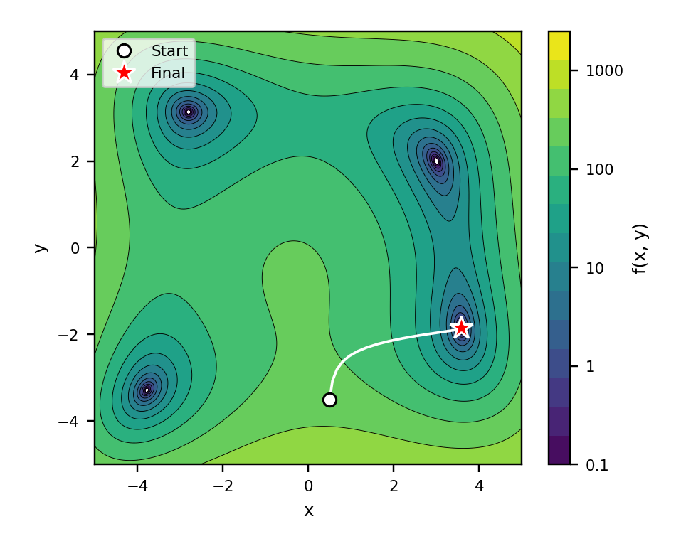
Fig. 6. Contours of a test function with an optimization path, start point, and final point.
Step 7: Export for Journals
- Size the figure at its final width: about 3.5 in (89 mm) for one IEEE column, and around 90 mm or 190 mm for Elsevier.
- Keep text at 7 to 9 pt at final size (Fig. 7).
- Export contours and line art as vector PDF or EPS. For very dense 3D surfaces, rasterize the surface or export a 600 dpi image, so the PDF stays light.
- Embed fonts, and check the dpi against the journal's artwork rules.
- Save your script and data with the figure, because revisions always come.
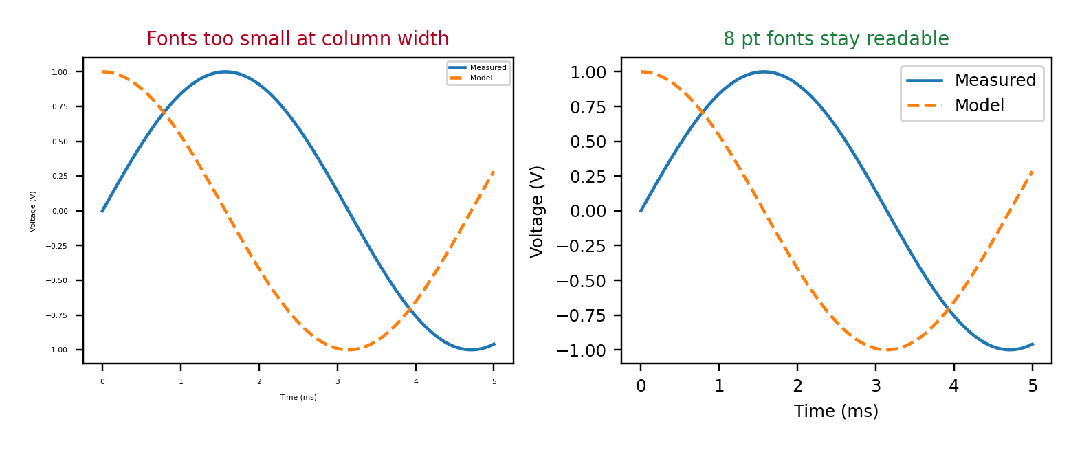
Fig. 7. Same figure width: tiny fonts fail at column width, 8 pt fonts stay readable.
Common Mistakes
- Leaving the default rainbow map in place.
- Missing colorbar labels, units, or axis labels.
- Using 3D where a 2D plot would be clearer.
- Taking screenshots instead of exporting vector files.
- Different color limits or view angles across panels that readers compare.
Final Checklist
- The plot type matches the question the figure answers.
- The color map is perceptually uniform and passes a grayscale test.
- Axes, colorbar, and units are labeled, and the text is 7 to 9 pt at final size.
- The figure is exported as vector, or at 600 dpi where raster is needed.
- The script, data, and final figure are saved together.
References
- E. R. Tufte, The Visual Display of Quantitative Information, 2nd ed. Cheshire, CT, USA: Graphics Press, 2001.
- J. D. Hunter, "Matplotlib: A 2D graphics environment," Computing in Science & Engineering, vol. 9, no. 3, pp. 90-95, 2007.
- C. R. Harris et al., "Array programming with NumPy," Nature, vol. 585, pp. 357-362, 2020.
- MathWorks, "MATLAB documentation: Graphics and 3-D visualization," mathworks.com.
- D. Borland and R. M. Taylor II, "Rainbow color map (still) considered harmful," IEEE Computer Graphics and Applications, vol. 27, no. 2, pp. 14-17, 2007.
- F. Crameri, G. E. Shephard, and P. J. Heron, "The misuse of colour in science communication," Nature Communications, vol. 11, Art. no. 5444, 2020.
- J. R. Nunez, C. R. Anderton, and R. S. Renslow, "Optimizing colormaps with consideration for color vision deficiency to enable accurate interpretation of scientific data," PLoS ONE, vol. 13, no. 7, Art. no. e0199239, 2018.
- B. Wong, "Points of view: Color blindness," Nature Methods, vol. 8, no. 6, p. 441, 2011.
- Elsevier, "Artwork and media instructions," Elsevier Author Resources.
Need Help with Publication-Quality Figures?
Get expert Python/MATLAB visualization support and formatting overhaul from ScholarGrid consultants.
Direct Email: scholargrid030@gmail.com